Data Handling - Importing CSV and Tabular data files in R Language

Setting up directories

→ We can change the current working directory as follows:
> setwd ("<location of the dataset>")

Example:
> setwd ("C":/RCourse/")
or
> setwd ("C:\\RCourse\\")

→ The following command returns the current working directory:

> getwd ( )
[1] "C:/RCourse/"

Importing Data Files

Suppose we have some data on our computer and we want to import it in R.

Different formats of files can be read in R

• comma-separated values (CSV) data files,
• table file (TXT)
• Spreadsheet (e.g., MS Excel) file,
• files from other software like SPSS, Minitab etc.

One can also read or upload the file from Internet site.

We can read the file containing rent index data from website:
http://home.iitk.ac.in/~shalab/Rcourse/munichdata.asc

as follows

> datamunich <- read.table (file = 
"http://home.iitk.ac.in/~shalab/Rcourse/munichdata.asc", header = TRUE)

File name is munichdata.asc

Comma-seperate values (CSV) files

First set the working directory where the CSV file is located.
setwd ("<location of your dataset>")

>setwd ("C:/RCourse/")

To read a CSV file
syntax: read.CSV ("filename.CSV")

Example:
> data <- read.CSV ("examplel.CSV")

Comma-separated values (CSV) files

Example:
> data <- read.CSV ("examplel.CSV")
> data
      X1    X10   X100
 1      2       20      200
 2      3       30      300
 3      4       40      400
 4      5       50      500

 Notice the difference in the first rows of excel file and output

Comma-separated values (CSV) files

Data files have many formats and accordingly we have options for loading them.

If the data file does not have headers in the first row, then use

data <- read.CSV ("datafile.CSV", header=FALSE)

Comma-separated values (CSV) files
The  resulting data frame will have columns named V1, V2, ...
We can rename the header names manually:

Comma-separated values (CSV) files
We can set the delimiter with sep.
If it is tab delimited, use  sep="\t".
data <- read.CSV ("datafile.CSV", sep="\t")

If it is space-delimited, use sep=" ".
data <- read.CSV ("datafile.CSV", sep= "  ") 

Reading Tabular Data Files

Tabular data files are test files with a simple format:

• Each linee contains one record.
• Within each record, fields (items) are separated by a one-character delimiter, such as a space, tab, colon, or comma.
• Each record contains the same number of fields.

we want to read a text file that contains a table of data.
read.table function is used and it returns a data frame.
read.table ("FileName") 

Read More

Basic of Calculations _Functions_Matrices in R Language

Function :-

Function are a bunch of commands grouped together in a sensible unit.

Functions take input arguments, do calculations (or make some graphics, call other functions) and produce some output and return a result in a variable. The returned variable can be a complex construct, like a list.

Syntax 

Name <- function(Argument1, Argument2, ...)
                {
                   expression
                                     }
Where expression is a single command or a group of commands

• Function arguments can be given a meaningful name
• Function arguments can be set to default values
• Functions can have the special argument '...'

Functions (Single variable)

The sign <- is furthermore used for defining functions:
> abc <- function(x) {
                    x^2
                         }

> abc (3)
  [1]  9

>abc (6)
  [1]  36

> abc (-2)
  [1]   4

Function (Two variables)

>abc  <- function (x,y) {
               x^2+y^2
                      }
> abc (2,3)
   [1]  13
> abc (3,4)
    [1]  25
> abc  (-2,-1)
   [1]  5

Matrix

• Matrices are important objects in any calculation.
• A matrix is a rectangular array with p rows and n columns.
• An element in the i-th row and j-th column is denoted by xij (book version) or x[i,j] ("program version"), i = 1,2,.....,n, j = 1,2,...,p. 
• An element of a matrix can also be an object, for example a string. However, in mathematics, we are mostly interested in numerical matrices, whose element are generally real numbers

In R, a 4⤫2-matrix x can be created with a following command:

>x <- matrix (nrow = 4 , ncol = 2, data = c(1,2,3,4,5,6,7,8) )

We see:

• The parameter nrow defines the row number of a matrix.
• The parameter ncol defines the column number of a matrix.
• The parameter data assigns specified values to the matrix element.
• The value from the parameters are written column-wise in matrix.

>  x
              [,1]          [,2]
[1,]           1             5
[2,]           2             6
[3,]           3             7
[4,]           4             8

• One can access a single element of a matrix with x[i,j] :

> x [3,2]
 [1]   7

Read More

Data Frames in R Programming

The commands c, cbind, vector and matrix functions combine data.

Another option is the data frame.

In a data frame, we can combine variables of equal length, which each row in the data frame containing observations on the same unit.

Hence, it is similar to the matrix or cbind functions.

Advantage is that one can make changes to the data without affecting the original data.

One can also combine numerical variables, character strings as well as factor in data frame.

For example, cbind and matrix functions can not be used to combine different types to data.

Data frames are special types of objects in R designed for data sets.

The data frame is similar to a spreadsheet, where columns contain variables and observations are contained in rows.

Data frames contain complete data sets that are mostly created with other programs (spreadsheet-files, software SPSS-files, Excel-files etc.).

Variables in a data frame may be numeric (numbers) or categorical (characters or factors).

Example :
Package "MASS" describes functions and data-sets to support Venables and Ripley, "Modern Applied Statistics with S" (4th edition 2002)

An example data frame Painters is available in the library.

MASS (here only an excerpt of a data set):

Here, the frames of the painters serve as row identifications, i.e.,
every row is assigned to the name of the corresponding painter.

Read More

String - Display and Splitting in R Language

Operations with Strings

Command strsplit, split the element of a character vector.

"Split" can be a single character, or a character string:

Usage 
strsplit (x,  split,  fixed = FALSE, ...)

Arguments
 x              character vector, each element of which is to be split.
 split    character vector containing regular expression(s) (unless fixed = TRUE) to use for splitting.

With a command strsplit, we can split a string in pieces.

> x <-  "The&! syntax&! of&! paste&! is&! !&available!& in the online-help"
> x 
[1]  "The&! syntax&! of&! paste&! is&! !&available!& in the online-help"

> strsplit (x , " ! ")
 [ [1] ]
 [1]     "The&"        "syntax&"       "of&"
 [4]     "paste&"      "is"                  "available"
 [7]     "&inthe online-help"

Read More

String - Display and Formatting in R Language

Strings

• Formatting and Display of Strings
• Operations with Strings

We need formatting and display of strings to obtain the results of specific operations in required format.

Formatting and Display of Strings

Important commands regarding formatting and display are
print , format , cat and  paste

print function prints its argument.

Usage
print ( )

print ( ) is a generic command that is available for every object class.

Examples:
> print (sqrt(2) )
 [1]  1.414214

> print ( sqrt (2) , digits = 5)
  [1] 1.4142

Format an R object for pretty printing.

Usage
format (x, ...)
x is any R object; typically numeric.

format (x, trim = FALSE, digits = NULL, nsmall = OL, justify = c("left" , "right" , "center" , "none") , width = NULL, . . .)

digits→shows how many significant digits are to be used.
nsmal→shows the minimum number of digits to the right of the decimal point.
justify→provides left-justified (the default), right-justified, or centered.

Examples:
> print (format ( 0.5, digits = 10, nsmall = 15) )
 [1]  "0.500000000000000"

Matrix display

> x <- matrix (nrow = 3, ncol = 2, data = 1:6, byrow = T)
> print (x)
          [,1]   [,2]
[1,]       1      2
[2,]       3      4
[3,]       5      6

Here, a matrix is displayed in the R command window.
One can specify the desired number of digits with the option digits.

The print function has a significant limitation that it prints only one object at a time.

Trying to print multiple items gives error message:

> print ("The zero occurs at", 2*pi, "radians.") Error in print.default("The zero occurs at",2*pi, "radians.") :
     invalid 'quote'  argument

The only way to print multiple items is to print them one at a time

> print ("The zero occurs at"); print (2*pi) ; print ("radians")
 [1]  "The zero occurs at"
 [1]  6.283185
 [1]  "radians"

The cat function is an alternative to print that lets you combine multiple items into a continuous output.

Read More

Data Management : Factors in R Language

Categorical variables

Quantitative variables
Example:
Height (in meters) - 1.65, 1.76, ....

Qualitative variables
Example:
Gender - Male, Female
Performance - Excellent, Good, Average, Bad ....

Categorical variables
Example:
x : Gender - Male, Female
x = 0 if a person is male
x = 1 if a person is female

Example:

The categories are stored internally as numeric codes, with labels to provide meaningful names for each code.

Factors

Factors represent categorical variables and are used as grouping indicators.

Example:
Suppose we denote the three colors of balls in a basket by following numbers:
Red = 1,  Blue = 2,  Green = 3

Suppose we draw five balls with following colors:
Red, Green, Green, Blue, Red

This outcome of colors can be coded by numbers

Each character is mapped to a code.

Factors represent categorical variables and are used as grouping indicators.

The categories are stored internally as numeric codes, with labels to provide meaningful names for each code.

The order of the labels is important.
First label is mapped to code 1.
Second label is mapped to code 2 and so on.

The values of the codes are always restricted to 1,2,...,k, to represent k discrete categories.

Here "Red" is mapped to code 1,
"Blue" is mapped to code 2 and 
"Green" is mapped to code 3.

We have a vector to character strings or integers.
R's term for a categorical variable is a factor.
In R, each possible value of a categorical variable is called a level.
A vector of level is called a factor.

A categorical variable is characterized by a (here : finite) number of levels called as factor levels.

To define a factor, we start with

• a vector of values,
• a second vector that gives the collection of possible values, and 
• a third vector that gives labels to the possible values.

A factor function encodes the vector of discrete values into a factor:
  factor (x)
          where x is a vector of strings or integers.
If the vector contains only a subset of possible values and not the entire values, then include a second argument that gives the possible levels of the factor:
  factor (x, levels)

Usage
factor (x = character ( ) , levels , labels = levels, exclude = NA, ..)

• levels : Determines the categories of the factor variable.                         Default is the sorted list of all the distinct values of x.
• labels : (Optionally Vector of values that will be the labels of the categories in the levels argument.
• exclude : (Optional) It defines which levels will be classified as NA in any output using the factor variable. 

Read More

Data Management : Vector indexing in R Language

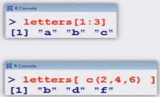
A vector of positive integers (letters, and Letters return the 26 lowercase and uppercase letters, respectively).

> letters [1 : 3]
 [1] "a"  "b"  "c"

> letters [c(2,4,6) ]
 [1]  "b"  "d"  "f'"

> LETTERS [1 : 3]
  [1]  "A"  "B"  "C"

> LETTERS [ c(2,4,6) ]
  [1]  "B"  "D"  "E"

> letters
 [1]  "a"  "b"  "c"  "d"  "e"  "f"  "g"  "h"  "i"  "j"  "k"  "l"  "m"  
[14] "n"  "o"  "p"  "q"  "r"  "s"  "t"  "u"  "v" "w"  "x"  "y"  "z" 
>
> LETTERS
 [1]  "A"  "B"  "C"  "D"  "E"  "F"  "G"  "H"  "I"  "J"  "K"  "L"  "M"
[14]  "N"  "O"  "P"  "Q"  "R"  "S"  "T"  "U"  "V"  "W"  "X"  "Y"  "Z"
>
> letters [1] 
 [1]  "a" 
>
> letters [14]
 [1]  "n"
>  Letters [1]
  [1]  "A"
> LETTERS [14]
 [1]  "N"
> letters [c(12,20,26) ]
 [1]  "1"  "t"  "z"


String vector
→ The elements of a vector can be named.
      Using these names, we can access the vector elements.

names is used for functions to get or set the names of an object.
> z <- list (al = 1, a2 = "c" , a3 = 1 :3)
> z
$al
 [1]  1
$a2
 [1]  "c"
$a3
 [1] 1 2 3

> names (z)
[1]  "a1"  "a2"  "a3"

Matrices created from Lists

List can be heterogeneous (mixed modes).
We can start with a heterogeneous list, give it dimensions, and thus create a heterogeneous matrix that is a mixture of numeric and character data:
Example
> ab  <- list (1, 2, 3, "x", "y" , "z")
> dim(ab)  <- c(2,3)
> print(ab)
      [,1]  [,2]  [,3]
[1,]   1     3      "y"
[2,]   2    "x"    "z"

Read More

Dataframes in R Language

Dataframes : Create dataframe

Data frames are generic data objects of R, used to store tabular data.

Code :-

# Introduction to data frames
 vec1 = c(1,2,3)
 vec2 = c("R","Scilab","Java")
 vec3 = c("For prototyping","For prototyping","For Scaleup")
 df = data.frame(vec1,vec2,vec3)
print(df)

Console Output

Create a dataframe using data from a file

• A dataframe can also be created by reading data from a file using the following command.        

                - newDF = read.table(path="Path of the file")

• In the path, please use '/' instead of '/' .

                - Example:  "C:/Users/hill/Documents/R/R-Workspace/"

• A separator can also be used to distinguish between entries. Default separator is space, ' ' .

               - newDF = read.table(file="path of the file" , sep)

Accessing rows and columns

• df[val1,val2] refers to row "val1" , column "val2" . Can be number or sting.
• "val1" or "val2" can also be array of values like "1:2" or "c(1,3)".
• df[val2] (no commas) - just refers to column "val2" only

Code :-

# accessing first & second row:
print(df[1:2,])
# accessing first & second column:
print(df[,1:2])
# accessing 1st & 2nd column -
# alternate:
print(df[1:2])

Output :-

Subset :-

Subset( ) which extracts subset of data based on conditions.

Editing dataframes

• A dataframe can also be edited using the edit( ) command
• Create an instance of data frame and use edit command to open a table editor, changes can be manually made.

Adding extra rows and columns

Extra row can be added with "rbind" function and extra column with "cbind".

Deleting rows and columns

There are several ways to delete a row/column, some cases are shown below.

Manipulating rows - the factor issue

• When character columns are created in a data .frame, they become factors
• Factor variables are those where the character column is split into categories or factor levels.

Resolving factor issue

New entries need to be consistent with factor levels which are fixed when the dataframe is first created.

Read More

Data Management : Lists in R Language

Vectors, matrices, and arrays is that each of these types of objects may only contain one type of data.

For example, a vector may contain all numeric data or all character data.

A list is a special type of object that can contain data of multiple types.

Lists are characterized by the fact that their element do not need to be of the same object type.

Lists can contain elements of different types so that the list elements may have different modes.

Lists can even contain other structured objects, such as lists and data frames which allows to create recursive data structures.

Lists can be indexed by position.
  So x [ [5] ] refers to the fifth element of x.

Lists can extract sublists.
 - So x [c (2,5) ] is a sublists of x that consists of the second and fifth elements.

Lists elements can have names.
 - Both x [ ["Students"] ] and x$Students refer to the element named "Students".

Difference between a vector and a list :

• In a vector, all element must have the same mode.
• In a list, the elements can have different modes.

Modes :

Every objects has a mode.

The mode indicates how the object is stored in memory: as a 

1. number
2. character string 
3. list of pointers to other objects,
4. function etc.

Mode function give us such information.

Syntax

mode ( )

Example

> mode (1.234)
 [1]  "numeric"

> mode ( c(5,6,7,8) )
  [1]  "numeric"

> mode ("India")
  [1]  "character"

> mode ( c( "India" , "USA") )
  [1]  "character"

  
Example

> mode (factor (c ("UP" , "MP") )   )
  [1]  "numeric "

> mode (list ("India", "USA") )
 [1]  "list"

>mode (data.frame (x=1:2, Y=c ("India", "USA" ) ) )
  [1]   "list"

> mode (print)
  [1]  "function"

Read More

Loops in R Language

The concept of executing a block of code multiples time.

Loops in R , are of following types

• For Loop : Executes statements multiple times, checks condition at the end.
• Repeat Loop : Repeats the code multiple times.
• While Loop : Executes code till a condition is satisfied.

For Loop :-
                     This loop iterates over a collection of values.

Syntax :-
                  for any_variable in collection_of_values
                     {
                            // Code to be executed
                      } 

Examples :-

While Loop :-
             Executes a set of statements till a condition is true,

Format :-
             While (Condition)
              {
                    // Code to be executed
               }

Examples :-

Repeat Loop :-
          A repeat loop executes a set of statements till a terminate statement is found.

The syntax of a repeat loop is :
                repeat
                         {
                              #Commands
                              if(condition)
                               {
                                   break
                                }
                          }

Examples :-

Read More

Analysis of Variance (ANOVA) and F-test in R Language

Analysis of Variance (ANOVA)

A statistical method for making simultaneous comparisons between two or more means; a statistical method that yields values that can be tested to determine whether a significant relation exists between variables.

Examples :-

A car company wishes to compare the average petrol consumption of THREE similar models of car and has available six vehicles of each model.

A teacher is interested in a comparison of average percentage marks attained in the examinations of FIVE different subjects and has available the marks of eight students who all completed each examination.

1. What ANOVA looks at is the way groups differ internally versus what the difference is between them. To take the above example:
2. ANOVA calculates the mean for each group.
3. It calculates the mean for all the group combined - the Overall Mean.
4. Then it calculates, within each group, the total deviation of each individual's score from the Group Mean - Within Group Variation.
5. Next, it calculates the deviation of each Group Mean from the Overall Mean - Between Group Variation.
6. Finally, ANOVA produces the F statistic which is the ratio - Between Group Variation to the Within Group Variation.
7. If the Between Group Variation is significantly greater than the Within Group Variation, then it is likely that there is a statistically significant difference between the groups.

One way Analysis of Variance

setwd("C:\\PERSONAL\\Irawen_Business_Analytics_With_R\\WIP\\Class-8 data-1")
data.ex1<-read.table("Class-8 data.txt",sep=',',head=T)
aov.ex1 = aov(Alertness~Dosage,data=data.ex1)
summary(aov.ex1) 

Two way Analysis of Variance

Data are from an experiment in which alertness level of male and female subjects was measured after they had been given one of two possible dosages of a drug. Thus, this is a 2x2 design with the factors being Gender and Dosage 



Used of Analysis of Variance

→ ANOVA is a particular form of statistical hypothesis testing heavily used in the analysis of experimental data.

→ A statistical hypothesis test is a method of making decisions using data. A test result (calculated from the null hypothesis and the sample) is called statistically significant if it is deemed unlikely to have occurred by chance, assuming the truth of the null hypothesis. A statistically significant result, when a probability (p-value) is less than a threshold (significance level), justifies the rejection of the null hypothesis, but only if the a priori probability of the null hypothesis is not high.

→In the typical application of ANOVA, the null hypothesis is that all groups are simply random samples of the same population. This implies that all treatments have the same effect (perhaps). Rejecting the null hypothesis implies that different treatments results in altered effects.   


More on ANOVA

ANOVA is the synthesis of several ideas and it is use for multiple purposes. As a consequence, it is difficult to define concisely or precisely.

Classical ANOVA for balanced data does three things at once:
- As exploratory data analysis, an ANOVA is an organization of an additive data decomposition, and its sums of squares indicate the variance of each component of the decomposition (or, equivalently, each set of terms of a linear model).
- Comparisons of mean squares, along with F-tests ... allow testing of a nested sequence of models.
- Closely related to the ANOVA is a linear model fit with coefficient estimates and standard errors. In short, ANOVA is a statistical tool used in several ways to develop and confirm an explanation for the observed data.

Additionally:

- It is computationally elegant and relatively robust against violations of its assumptions.
- ANOVA provides industrial strength (multiple sample comparison) statistical analysis.
- It has been adapted to the analysis os a variety of exprimental designs.

F-test

An F-test is any statistical test in which the test statistic has an F-distribution under the null hypothesis.

It is most often used when comparing statistical models that have been fitted to a data set, in order to identify the model that best fits the population from which the data were sampled.

Exact "F-test" mainly arise when the models have been fitted to the data using least squares.

The name was coined by George W. Snedecor, in honour of Sir Ronald A.Fisher.

Fisher initially developed the statistic as the variance ratio in the 1920s.

The formula for the one-way ANOVA F-test statistic is:

  

Read More

Decision Making in R Language

Decision Making

Decision Making structure, evaluate a condition and depending on the result some other code is processed.

There are three types of decision making statements in R

• If Statement
• If-Else Statement
• Switch Statement

If Statement

An if statement consists of a Boolean expression followed by one or more statement.

Syntax of is Statement :-

if(Boolean expression)
{
   // Code to be executed
}

If-Else Statements

An if statement can be followed by an optional else statement, which executes when the Boolean expression is false.

The syntax of if else is :

if (Boolean_expression)
{
   // Code to be executed
} 
else
{
    // Code to be executed
}

Example :-

   
Switch Statement

A switch statement allows a variable to be tested for equality against a list of values.

R has following Switch Statement :

    switch (expression, case1, case2..)
→ We can have any number of cases in switch.
→ No Default is available in switch.

Read More