Calculate Simple Interest in Android App

Activity_main.xml File

 <?xml version="1.0" encoding="utf-8"?> 

<LinearLayout xmlns:android="http://schemas.android.com/apk/res/android" 

 xmlns:app="http://schemas.android.com/apk/res-auto"     

xmlns:tools="http://schemas.android.com/tools" 

 android:layout_width="match_parent"     

android:layout_height="match_parent"     

android:orientation="vertical" 

 tools:context=".MainActivity">

<TextView 

 android:layout_width="fill_parent"         

android:layout_height="wrap_content" 

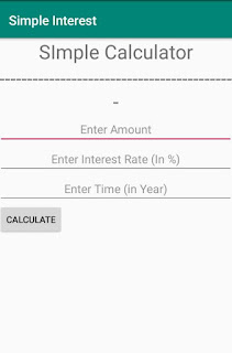
 android:text="SImple Calculator"         

android:textAlignment="center" 

 android:textSize="30dp"        />
 

<TextView         

android:layout_width="fill_parent" 

 android:layout_height="wrap_content" 

 android:text="------------------------------------------" 

 android:textAlignment="center"         

android:textSize="30dp"  />

<EditText         

android:layout_width="fill_parent" 

 android:layout_height="wrap_content" 

 android:hint="Enter Amount"         

android:id="@+id/amt" 

 android:textAlignment="center" 

 android:inputType="number"/>

<EditText         

android:layout_width="fill_parent" 

 android:layout_height="wrap_content"         

android:hint="Enter Interest Rate (In %)" 

 android:id="@+id/interest"         

android:textAlignment="center" 

 android:inputType="number"/>

<EditText 

 android:layout_width="fill_parent"         

android:layout_height="wrap_content" 

 android:hint="Enter Time (in Year)"         

android:id="@+id/tim" 

 android:textAlignment="center" 

 android:inputType="number"        />

<Button 

 android:layout_width="wrap_content"         

android:layout_height="wrap_content"         

android:text="Calculate" 

 android:id="@+id/btn"        />

<TextView         

android:layout_width="fill_parent"         

android:layout_height="wrap_content" 

 android:id="@+id/txt1"         

android:textSize="30dp"        />

    
<TextView         

android:layout_width="fill_parent" 

 android:layout_height="wrap_content" 

 android:id="@+id/txt2" 

 android:textSize="20dp"        />

</LinearLayout>

MainActivity.Java File

 
package com.irawen.simpleinterest;
import android.support.v7.app.AppCompatActivity;
import android.os.Bundle;
import android.view.View;
import android.widget.Button;
import android.widget.EditText;
import android.widget.TextView;

public class MainActivity extends AppCompatActivity {

    @Override    protected void onCreate(Bundle savedInstanceState) {
        super.onCreate(savedInstanceState);
        setContentView(R.layout.activity_main);

        OnCLick();
    }

    EditText amt,interest,time;
    Button btn;
    TextView txt1,txt2;

    public  void OnCLick()
    {
        amt=(EditText)findViewById(R.id.amt);
        interest=(EditText)findViewById(R.id.interest);
        time=(EditText)findViewById(R.id.tim);
        btn=(Button)findViewById(R.id.btn);
        txt1=(TextView)findViewById(R.id.txt1);
        txt2=(TextView)findViewById(R.id.txt2);

        btn.setOnClickListener(new View.OnClickListener() {
            @Override            public void onClick(View v) {
                int a=Integer.parseInt(amt.getText().toString());
                int b=Integer.parseInt(interest.getText().toString());
                int c=Integer.parseInt(time.getText().toString());
                int d;
                d=(a*b*c)/100;
                int e=a+d;

                txt1.setText("Total Interest Is :"+String.valueOf(d));
                txt2.setText("Total Amount is : "+String.valueOf(e));

            }
        });
    }
}

Read More

Random Forest in R Language

In the random forest approach, a large number of decision trees are created. Every observation is fed into every decision tree. The most common outcome for each observation is used as the final output. A new observation is fed into all the trees and taking a majority vote for each classification model.

An error estimate is made for the cases which were not used while building the tree. That is called an OOB (Out-of-bag) error estimate which is mentioned as a percentage.

The R package "randomForest" is used to create random forests.

Install R Package

Use the below command in R console to install the package. You also have to install the dependent packages if any.

install.packages("randomForest)

The package "randomForest" has the function randomForest() which is used to create and analyze random forests.

SYNTAX

The basic syntax for creating a random forest in R is −

randomForest(formula, data)

Following is the description of the parameters used −

• formula is a formula describing the predictor and response variables.
• data is the name of the data set used.

INPUT DATA

We will use the R in-built data set named readingSkills to create a decision tree. It describes the score of someone's readingSkills if we know the variables "age","shoesize","score" and whether the person is a native speaker.

Here is the sample data.

# Load the party package. It will automatically load other required packages.
library(party)

# Print some records from data set readingSkills.
print(head(readingSkills))

When we execute the above code, it produces the following result and chart −

  nativeSpeaker   age   shoeSize      score
1           yes     5   24.83189   32.29385
2           yes     6   25.95238   36.63105
3            no    11   30.42170   49.60593
4           yes     7   28.66450   40.28456
5           yes    11   31.88207   55.46085
6           yes    10   30.07843   52.83124
Loading required package: methods
Loading required package: grid
...............................
...............................

EXAMPLE

We will use the randomForest() function to create the decision tree and see it's graph.

# Load the party package. It will automatically load other required packages.
library(party)
library(randomForest)

# Create the forest.
output.forest <- randomForest(nativeSpeaker ~ age + shoeSize + score, 
           data = readingSkills)

# View the forest results.
print(output.forest) 

# Importance of each predictor.
print(importance(fit,type = 2)) 

When we execute the above code, it produces the following result −

Call:
 randomForest(formula = nativeSpeaker ~ age + shoeSize + score,     
                 data = readingSkills)
               Type of random forest: classification
                     Number of trees: 500
No. of variables tried at each split: 1

        OOB estimate of  error rate: 1%
Confusion matrix:
    no yes class.error
no  99   1        0.01
yes  1  99        0.01
         MeanDecreaseGini
age              13.95406
shoeSize         18.91006
score            56.73051

CONCLUSION

From the random forest shown above we can conclude that the shoe-size and score are the important factors deciding if someone is a native speaker or not. Also the model has only 1% error which means we can predict with 99% accuracy.

Read More

Logistic Regression in R Language

The Logistic Regression is a regression model in which the response variable (dependent variable) has categorical values such as True/False or 0/1. It actually measures the probability of a binary response as the value of response variable based on the mathematical equation relating it with the predictor variables.

The general mathematical equation for logistic regression is −

y = 1/(1+e^-(a+b1x1+b2x2+b3x3+...))

Following is the description of the parameters used −

• y is the response variable.
• x is the predictor variable.
• a and b are the coefficients which are numeric constants.

The function used to create the regression model is the glm() function.

Syntax

The basic syntax for glm() function in logistic regression is −

glm(formula,data,family)

Following is the description of the parameters used −

• formula is the symbol presenting the relationship between the variables.
• data is the data set giving the values of these variables.
• family is R object to specify the details of the model. It's value is binomial for logistic regression.

Example

The in-built data set "mtcars" describes different models of a car with their various engine specifications. In "mtcars" data set, the transmission mode (automatic or manual) is described by the column am which is a binary value (0 or 1). We can create a logistic regression model between the columns "am" and 3 other columns - hp, wt and cyl.

# Select some columns form mtcars.
input <- mtcars[,c("am","cyl","hp","wt")]

print(head(input))

When we execute the above code, it produces the following result −

                  am   cyl  hp    wt
Mazda RX4          1   6    110   2.620
Mazda RX4 Wag      1   6    110   2.875
Datsun 710         1   4     93   2.320
Hornet 4 Drive     0   6    110   3.215
Hornet Sportabout  0   8    175   3.440
Valiant            0   6    105   3.460

 

Create Regression Model

We use the glm() function to create the regression model and get its summary for analysis.

input <- mtcars[,c("am","cyl","hp","wt")]

am.data = glm(formula = am ~ cyl + hp + wt, data = input, family = binomial)

print(summary(am.data))

When we execute the above code, it produces the following result −

Call:
glm(formula = am ~ cyl + hp + wt, family = binomial, data = input)

Deviance Residuals: 
     Min        1Q      Median        3Q       Max  
-2.17272     -0.14907  -0.01464     0.14116   1.27641  

Coefficients:
            Estimate Std. Error z value Pr(>|z|)  
(Intercept) 19.70288    8.11637   2.428   0.0152 *
cyl          0.48760    1.07162   0.455   0.6491  
hp           0.03259    0.01886   1.728   0.0840 .
wt          -9.14947    4.15332  -2.203   0.0276 *
---
Signif. codes:  0 ‘***’ 0.001 ‘**’ 0.01 ‘*’ 0.05 ‘.’ 0.1 ‘ ’ 1

(Dispersion parameter for binomial family taken to be 1)

    Null deviance: 43.2297  on 31  degrees of freedom
Residual deviance:  9.8415  on 28  degrees of freedom
AIC: 17.841

Number of Fisher Scoring iterations: 8

 

CONCLUSION

In the summary as the p-value in the last column is more than 0.05 for the variables "cyl" and "hp", we consider them to be insignificant in contributing to the value of the variable "am". Only weight (wt) impacts the "am" value in this regression model.

Read More

Mean, Median & Mode in R Language

Statistical analysis in R is performed by using many in-built functions. Most of these functions are part of the R base package. These functions take R vector as an input along with the arguments and give the result.

The functions we are discussing in this chapter are mean, median and mode.

Mean

It is calculated by taking the sum of the values and dividing with the number of values in a data series.

The function mean() is used to calculate this in R.

The basic syntax for calculating mean in R is −

mean(x, trim = 0, na.rm = FALSE, ...)

Following is the description of the parameters used −

• x is the input vector.
• trim is used to drop some observations from both end of the sorted vector.
• na.rm is used to remove the missing values from the input vector.

EXAMPLE

# Create a vector. 
x <- c(12,7,3,4.2,18,2,54,-21,8,-5)

# Find Mean.
result.mean <- mean(x)
print(result.mean)

When we execute the above code, it produces the following result −

[1] 8.22

Applying Trim Option

When trim parameter is supplied, the values in the vector get sorted and then the required numbers of observations are dropped from calculating the mean.

When trim = 0.3, 3 values from each end will be dropped from the calculations to find mean.

In this case the sorted vector is (−21, −5, 2, 3, 4.2, 7, 8, 12, 18, 54) and the values removed from the vector for calculating mean are (−21,−5,2) from left and (12,18,54) from right.

# Create a vector.
x <- c(12,7,3,4.2,18,2,54,-21,8,-5)

# Find Mean.
result.mean <-  mean(x,trim = 0.3)
print(result.mean)

When we execute the above code, it produces the following result −

[1] 5.55

Applying NA Option

If there are missing values, then the mean function returns NA.

To drop the missing values from the calculation use na.rm = TRUE. which means remove the NA values.

# Create a vector. 
x <- c(12,7,3,4.2,18,2,54,-21,8,-5,NA)

# Find mean.
result.mean <-  mean(x)
print(result.mean)

# Find mean dropping NA values.
result.mean <-  mean(x,na.rm = TRUE)
print(result.mean)

When we execute the above code, it produces the following result −

[1] NA
[1] 8.22

 

Median

The middle most value in a data series is called the median. The median() function is used in R to calculate this value.

SYNTAX

The basic syntax for calculating median in R is −

median(x, na.rm = FALSE)

Following is the description of the parameters used −

• x is the input vector.
• na.rm is used to remove the missing values from the input vector.

EXAMPLE

# Create the vector.
x <- c(12,7,3,4.2,18,2,54,-21,8,-5)

# Find the median.
median.result <- median(x)
print(median.result)

When we execute the above code, it produces the following result −

[1] 5.6

 

Mode

The mode is the value that has highest number of occurrences in a set of data. Unike mean and median, mode can have both numeric and character data.

R does not have a standard in-built function to calculate mode. So we create a user function to calculate mode of a data set in R. This function takes the vector as input and gives the mode value as output.

EXAMPLE

# Create the function.
getmode <- function(v) {
   uniqv <- unique(v)
   uniqv[which.max(tabulate(match(v, uniqv)))]
}

# Create the vector with numbers.
v <- c(2,1,2,3,1,2,3,4,1,5,5,3,2,3)

# Calculate the mode using the user function.
result <- getmode(v)
print(result)

# Create the vector with characters.
charv <- c("o","it","the","it","it")

# Calculate the mode using the user function.
result <- getmode(charv)
print(result)

When we execute the above code, it produces the following result −

[1] 2
[1] "it"

Read More

Nonlinear Least Square in R Language

 Nonlinear Least Square

When modeling real world data for regression analysis, we observe that it is rarely the case that the equation of the model is a linear equation giving a linear graph. Most of the time, the equation of the model of real world data involves mathematical functions of higher degree like an exponent of 3 or a sin function. In such a scenario, the plot of the model gives a curve rather than a line. The goal of both linear and non-linear regression is to adjust the values of the model's parameters to find the line or curve that comes closest to your data. On finding these values we will be able to estimate the response variable with good accuracy.

In Least Square regression, we establish a regression model in which the sum of the squares of the vertical distances of different points from the regression curve is minimized. We generally start with a defined model and assume some values for the coefficients. We then apply the nls() function of R to get the more accurate values along with the confidence intervals.

Syntax

The basic syntax for creating a nonlinear least square test in R is −

nls(formula, data, start)

Following is the description of the parameters used −

• formula is a nonlinear model formula including variables and parameters.
• data is a data frame used to evaluate the variables in the formula.
• start is a named list or named numeric vector of starting estimates.

Example

We will consider a nonlinear model with assumption of initial values of its coefficients. Next we will see what is the confidence intervals of these assumed values so that we can judge how well these values fir into the model.

So let's consider the below equation for this purpose −

a = b1*x^2+b2

Let's assume the initial coefficients to be 1 and 3 and fit these values into nls() function.

xvalues <- c(1.6,2.1,2,2.23,3.71,3.25,3.4,3.86,1.19,2.21)
yvalues <- c(5.19,7.43,6.94,8.11,18.75,14.88,16.06,19.12,3.21,7.58)

# Give the chart file a name.
png(file = "nls.png")


# Plot these values.
plot(xvalues,yvalues)


# Take the assumed values and fit into the model.
model <- nls(yvalues ~ b1*xvalues^2+b2,start = list(b1 = 1,b2 = 3))

# Plot the chart with new data by fitting it to a prediction from 100 data points.
new.data <- data.frame(xvalues = seq(min(xvalues),max(xvalues),len = 100))
lines(new.data$xvalues,predict(model,newdata = new.data))

# Save the file.
dev.off()

# Get the sum of the squared residuals.
print(sum(resid(model)^2))

# Get the confidence intervals on the chosen values of the coefficients.
print(confint(model))

When we execute the above code, it produces the following result −

[1] 1.081935
Waiting for profiling to be done...
       2.5%    97.5%
b1 1.137708 1.253135
b2 1.497364 2.496484

We can conclude that the value of b1 is more close to 1 while the value of b2 is more close to 2 and not 3.

Read More

Time Series Analysis in R Language

Time series is a series of data points in which each data point is associated with a timestamp. A simple example is the price of a stock in the stock market at different points of time on a given day. Another example is the amount of rainfall in a region at different months of the year. R language uses many functions to create, manipulate and plot the time series data. The data for the time series is stored in an R object called time-series object. It is also a R data object like a vector or data frame.

The time series object is created by using the ts()function.

Syntax

The basic syntax for ts() function in time series analysis is −

timeseries.object.name <-  ts(data, start, end, frequency)

Following is the description of the parameters used −

• data is a vector or matrix containing the values used in the time series.
• start specifies the start time for the first observation in time series.
• end specifies the end time for the last observation in time series.
• frequency specifies the number of observations per unit time.

Except the parameter "data" all other parameters are optional.

Example

Consider the annual rainfall details at a place starting from January 2012. We create an R time series object for a period of 12 months and plot it.

# Get the data points in form of a R vector.
rainfall <- c(799,1174.8,865.1,1334.6,635.4,918.5,685.5,998.6,784.2,985,882.8,1071)

# Convert it to a time series object.
rainfall.timeseries <- ts(rainfall,start = c(2012,1),frequency = 12)

# Print the timeseries data.
print(rainfall.timeseries)

# Give the chart file a name.
png(file = "rainfall.png")

# Plot a graph of the time series.
plot(rainfall.timeseries)

# Save the file.
dev.off()

When we execute the above code, it produces the following result and chart −

Jan    Feb    Mar    Apr    May     Jun    Jul    Aug    Sep
2012  799.0  1174.8  865.1  1334.6  635.4  918.5  685.5  998.6  784.2
        Oct    Nov    Dec
2012  985.0  882.8 1071.0

The Time series chart −

Different Time Intervals

The value of the frequency parameter in the ts() function decides the time intervals at which the data points are measured. A value of 12 indicates that the time series is for 12 months. Other values and its meaning is as below −

• frequency = 12 pegs the data points for every month of a year.
• frequency = 4 pegs the data points for every quarter of a year.
• frequency = 6 pegs the data points for every 10 minutes of an hour.
• frequency = 24*6 pegs the data points for every 10 minutes of a day.

Multiple Time Series

We can plot multiple time series in one chart by combining both the series into a matrix.

# Get the data points in form of a R vector.

 rainfall1 <- c(799,1174.8,865.1,1334.6,635.4,918.5,685.5,998.6,784.2,985,882.8,1071)
rainfall2 <- 
           c(655,1306.9,1323.4,1172.2,562.2,824,822.4,1265.5,799.6,1105.6,1106.7,1337.8)

# Convert them to a matrix.
combined.rainfall <-  matrix(c(rainfall1,rainfall2),nrow = 12)

# Convert it to a time series object.
rainfall.timeseries <- ts(combined.rainfall,start = c(2012,1),frequency = 12)

# Print the timeseries data. print(rainfall.timeseries)

# Give the chart file a name.
png(file = "rainfall_combined.png")

# Plot a graph of the time series.
plot(rainfall.timeseries, main = "Multiple Time Series")

# Save the file.
dev.off()

When we execute the above code, it produces the following result and chart −

           Series 1  Series 2
Jan 2012    799.0    655.0
Feb 2012   1174.8   1306.9
Mar 2012    865.1   1323.4
Apr 2012   1334.6   1172.2
May 2012    635.4    562.2
Jun 2012    918.5    824.0
Jul 2012    685.5    822.4
Aug 2012    998.6   1265.5
Sep 2012    784.2    799.6
Oct 2012    985.0   1105.6
Nov 2012    882.8   1106.7
Dec 2012   1071.0   1337.8

The Multiple Time series chart −

Read More