Basics Calculations: Matrix Operations in R Language

In R, a 4 𝗑 2-matrix X can be created with a following command:

> x <-  matrix (nrow=4,   ncol=2,  data=c(1,2,3,4,5,6,7,8)  )

> x
                [,1]       [,2]
[1,]             1          5
[2,]             2          6
[3,]             3          7
[4,]             4          8

Properties of a Matrix

We can get specific properties of a matrix:


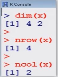
> dim (x)         # tells the
[1]   4   2             dimension of matrix

> nrow (x)       # tells
[1]  4                    the number of rows

> ncol (x)        # tells 
[1]  2                  the number of columns

> mode (x)      # Informs the type or storage mode of an object, e.g., numerical, logical etc.

[1]   "numeric"

attributes provides all the attributes of an object

> attributes (x)    # Informs the dimension of matrix 

$dim   [1]    4   2

Help on the Object "Matrix"

To know more about these important objects, we use R-help on "matrix".

> help ("matrix")

matrix     package:base            R Documentation

Matrices

Description :

'matrix'  creates a matrix from the given set of values.

'as.matrix' attempts to turn its argument into a matrix.

'is.matrix'  tests if its argument is a (strict) matrix. It is generic: you can write methods to handle specific classes of objects, see Internal Methods.

Then we get an overview on how a matrix can be created and what parameters are available:

Usage :

   matrix(data  [= NA, nrow = 1 , ncol = 1, byrow = FALSE, dimension = NULL)

  as.matrix (x)

  is. matrix (x)

Arguments :

  data: an optional data vector.

  nrow: the desired number of rows

  ncol: the desired number of columns

  byrow: logical. If 'FALSE' (the default) the matrix is filled by columns, otherwise the matrix is filled by rows.

dimnames:  A 'dimnames'  attribute for the matrix: a 'list' of length 2.

        x: an R object.

Finally, references and cross-references are displayed...

References :

  Becker, R. A.,  Chambers, J. M. and wilks, A.

  R. (1988)  _The New S Language_. wadsworth & Books/Cole.

See Also:

  'data.matrix' , which attempts to convert to a numeric matrix.

.... as well as an example:

Examples :

  is.matrix (as.matrix (1 : 10) )

  data (warpbreaks)

  ! is.matrix(warpbreaks) #  data.frame, NOT matrix!

  warpbreaks [1 : 10,]

  as.matrix(warpbreaks[1 : 10,])  #using

      as.matrix.data.frame(.) method

Matrix Operations 

Assigning a specified number to all matrix elements:

> x  <-  matrix (nrow=4, ncol=2, data=2 )

> x 

             [,1]    [,2]

[1,]         2        2

[2,]         2        2

[3,]         2        2

[4,]         2        2

Construction of a diagonal matrix, here the identity matrix of a dimension 2:

> d  <-  diag (1,  nrow=2,  ncol=2)

> d

        [,1]   [,2]

[1,]    1       0

[2,]    0       1

Transpose of a matrix x:  x'

>  x  <- matrix (nrow=4, ncol=2, data=1:8,  byrow=T )

>  x

                [,1]      [,2]

[1,]             1          2

[2,]             3          4

[3,]             5          6

[4,]             7          8

Multiplication of a matrix with a constant

Read More

Statistical Functions - Central Tendency and Variation in R language

Descriptive statistics :-

First hand tools which gives first hand information.

• Central tendency of data (Mean, median, mode, geometric mean, harmonic mean etc.)
• Variation in data (variance, standard deviation, standard error, mean deviation etc.)

Central tendency of the data

Gives an idea about the mean value of the data 
The data is clustered around what value?

Data:  𝒳1, 𝒳2, ......,𝒳n
x : Data vector

mean (x)

 prod (x) ^ (1/length (x) )
(length (x)  is equal to the number of elements in x)

Median :-

     Value such that the number of observation above it is equal to the number of observation below it.
median (x)

Example :-

Variability

spread and scatterdness of data around any point, preferably the mean value.

Data set 1:  360, 370, 380
    mean = (360 + 370 + 380) /3  = 370
Data set 2:  10, 100, 1000
    mean = (10 + 100 + 1000) /3  = 370

How to differentiate between the two data sets?

  x : data vector
      var (x)
positive square root of variance : standard deviation
        sqrt (var (x) )

Variance
Another variant,

If we want divisor to be n, then use
   ( (n-1) /n) * var (x)
where  n = length (x)

Range:
    maximum(x1, x2, ....., xn) - minimum(x1, x2, ...., xn)
      max (x)  -  min (x)

Interquartile range:
  Third quartile (x1, x2, ..., xn) - First quartile (x1, x2, ...., xn)
     IQR (x)

Quartile deviation:
  [Third quartile (x1, x2, ..., xn) - First quartile (x1, x2, ..., xn)]/2
   =  Interquartile range/2
    IQR (x) /2


Example :-

Read More

Statistical Functions - Graphics and Plots in R Language

Graphics tools :

Graphics tools - various type of plots

• 2D & 3D plots,
• scatter diagram
• Pie diagram
• Histogram
• Bar plot
• Stem and leaf plot
• Box plot ....

Appropriate number and choice of plots in analysis provides better inferences.

In R, such graphics can be easily created and saved in various formats.

• Bar plot
• Pie chart
• Box plot
• Grouped box plot
• Scatter plot
• Coplots
• Histogram
• Normal QQ plot ...

Bar plots :-

→ Visualize the relative or absolute frequencies of observed values of a variable.
→ It consists of one bar for each category.
→ The height of each bar is determined by either the absolute frequency or the relative frequency of the respective category and is shown on the y-axis.

barplot (x, width = 1, space = NULL ,...)
> barplot (table (x) )
> barplot (table (x) / length (x) )

Example :-
Code the 10 persons by using, say 1 for male (M) and 2 for female (F).
  M, F, M, F, M, M, M, F, M, M
   1,  2, 1,  2,  1,  1,   1,  2,  1,  1

> gender <-  c(1, 2, 1, 2, 1, 1, 1, 2, 1, 1) 
> gender
 [1]  1  2  1  2  1  1  1  2  1  1

Example :-
> barplot (gender)
Do you want this ?
2 categories 
M = 7
F  = 3

Pie diagram :-

Pie charts visualize the absolute and relative frequencies.

A pie chart is a circle partitioned into segments where each of the segments represents a category.

The size of each segment depends upon the relative frequency and is determined by the angle (frequency x 360 degree).

pie (x,  labels  = names (x),  ...)

Example :-

> pie (gender)

Histogram :-

Histogram is based on the idea to categorize the data into different groups and plot the bars for each category with height.

The area of the bar (= height x width ) is proportional to the relative frequency.

So the width of the bars need not necessarily to be the same

hist (x)  # show absolute frequencies 
hist (x, freq=F)   # show relative frequencies

see help ("hist") for more details

Read More

Statistical Functions : Frequency and Partition values in R Language

Descriptive statistics:

First hand tools which gives first hand information

• Central tendency of data
• Variation in data
• Structure and shape of data tendency
• Relationship study

Graphical as well as analytical tools are used.

Absolute and relative frequencies:

Suppose there are 10 persons coded into two categories as male (M) and female (F).
   M, F, M, F, M, M, M, F, M, M,

Use a1 and a2 to refer to male and female categories.

There are 7 male and 3 female persons, denoted as n1 = 7 and n2 = 3
The number of observations in a particular category is called the absolute frequency.

The relative frequencies of a1 and a2 are
  f1 = n1/ n1 + n2
      =  7/10
      = 0.7
      = 70%
 f2  = n2/n1 + n2
      = 3/10
      = 0.3
      =  30% 
This gives us information about the propotions of male and female persons.

table (variable) create the sample frequency of the variable of the data file.

Enter data as x
table (x)   # absolute frequencies
table (x) / length (x)   # relative frequencies

Example: Code the 10 persons by using, say 1 for male (M and 2 for female (F).
          M, F, M, F, M, M, M, F, M, M 
           1,  2, 1,  2,  1,   1,  1,  2,  1,   1
> gender <-   c(1, 2, 1, 2, 1, 1, 1, 2, 1, 1)
>gender
  [1]     1 2 1 2 1 1 1 2 1 1

> table (gender)  # Absolute frequencies
 gender
   1   2
   7   3
 

> table (gender) / length (gender)   #Relative freq. gender
   1     2
 0.7   0.3

Example:

'Pizza_delivery.csv'  contains the simulated data on pizza home delivery.

•  There are three branches (East, West, Central)  of the restaurant.
• The pizza delivery in centrally managed over phone and delivered by one of the five drivers.
• The data set captures the number of pizzas ordered and the final bill.

> setwd ("C: / Resource")
> pizza <- read.csv (' pizza_delivery.csv ' )

Example :

Consider data from pizza. Take first 100  values  from Direction and code Directions as 

1. East: 1
2. West: 2
3. Center: 3

Partition values:

Such values divides the total frequency given data into required number of partitions.

Quartile:  Divides the data into 4 equal parts.
Decile:  Divides the data into 10 equal parts.
Percentile:  Divides the data into 100 equal parts.

quantile function computes quantiles corresponding to the given probabilities.
The smallest observation corresponds to a probability of 0 and thr largest to a probability of 1.

quantile (x, . . . .)
quantile(x, probs = seq(0, 1, 0.25, . . .)

Arguments
x           numeric vector whose sample quantile are wanted,
probs    numeric vector of probabilities with values in [0,1]. 

Example:  Marks of 15 students are

Read More

Data Handling - Importing CSV and Tabular data files in R Language

Setting up directories

→ We can change the current working directory as follows:
> setwd ("<location of the dataset>")

Example:
> setwd ("C":/RCourse/")
or
> setwd ("C:\\RCourse\\")

→ The following command returns the current working directory:

> getwd ( )
[1] "C:/RCourse/"

Importing Data Files

Suppose we have some data on our computer and we want to import it in R.

Different formats of files can be read in R

• comma-separated values (CSV) data files,
• table file (TXT)
• Spreadsheet (e.g., MS Excel) file,
• files from other software like SPSS, Minitab etc.

One can also read or upload the file from Internet site.

We can read the file containing rent index data from website:
http://home.iitk.ac.in/~shalab/Rcourse/munichdata.asc

as follows

> datamunich <- read.table (file = 
"http://home.iitk.ac.in/~shalab/Rcourse/munichdata.asc", header = TRUE)

File name is munichdata.asc

Comma-seperate values (CSV) files

First set the working directory where the CSV file is located.
setwd ("<location of your dataset>")

>setwd ("C:/RCourse/")

To read a CSV file
syntax: read.CSV ("filename.CSV")

Example:
> data <- read.CSV ("examplel.CSV")

Comma-separated values (CSV) files

Example:
> data <- read.CSV ("examplel.CSV")
> data
      X1    X10   X100
 1      2       20      200
 2      3       30      300
 3      4       40      400
 4      5       50      500

 Notice the difference in the first rows of excel file and output

Comma-separated values (CSV) files

Data files have many formats and accordingly we have options for loading them.

If the data file does not have headers in the first row, then use

data <- read.CSV ("datafile.CSV", header=FALSE)

Comma-separated values (CSV) files
The  resulting data frame will have columns named V1, V2, ...
We can rename the header names manually:

Comma-separated values (CSV) files
We can set the delimiter with sep.
If it is tab delimited, use  sep="\t".
data <- read.CSV ("datafile.CSV", sep="\t")

If it is space-delimited, use sep=" ".
data <- read.CSV ("datafile.CSV", sep= "  ") 

Reading Tabular Data Files

Tabular data files are test files with a simple format:

• Each linee contains one record.
• Within each record, fields (items) are separated by a one-character delimiter, such as a space, tab, colon, or comma.
• Each record contains the same number of fields.

we want to read a text file that contains a table of data.
read.table function is used and it returns a data frame.
read.table ("FileName") 

Read More

Basic of Calculations _Functions_Matrices in R Language

Function :-

Function are a bunch of commands grouped together in a sensible unit.

Functions take input arguments, do calculations (or make some graphics, call other functions) and produce some output and return a result in a variable. The returned variable can be a complex construct, like a list.

Syntax 

Name <- function(Argument1, Argument2, ...)
                {
                   expression
                                     }
Where expression is a single command or a group of commands

• Function arguments can be given a meaningful name
• Function arguments can be set to default values
• Functions can have the special argument '...'

Functions (Single variable)

The sign <- is furthermore used for defining functions:
> abc <- function(x) {
                    x^2
                         }

> abc (3)
  [1]  9

>abc (6)
  [1]  36

> abc (-2)
  [1]   4

Function (Two variables)

>abc  <- function (x,y) {
               x^2+y^2
                      }
> abc (2,3)
   [1]  13
> abc (3,4)
    [1]  25
> abc  (-2,-1)
   [1]  5

Matrix

• Matrices are important objects in any calculation.
• A matrix is a rectangular array with p rows and n columns.
• An element in the i-th row and j-th column is denoted by xij (book version) or x[i,j] ("program version"), i = 1,2,.....,n, j = 1,2,...,p. 
• An element of a matrix can also be an object, for example a string. However, in mathematics, we are mostly interested in numerical matrices, whose element are generally real numbers

In R, a 4⤫2-matrix x can be created with a following command:

>x <- matrix (nrow = 4 , ncol = 2, data = c(1,2,3,4,5,6,7,8) )

We see:

• The parameter nrow defines the row number of a matrix.
• The parameter ncol defines the column number of a matrix.
• The parameter data assigns specified values to the matrix element.
• The value from the parameters are written column-wise in matrix.

>  x
              [,1]          [,2]
[1,]           1             5
[2,]           2             6
[3,]           3             7
[4,]           4             8

• One can access a single element of a matrix with x[i,j] :

> x [3,2]
 [1]   7

Read More

Data Frames in R Programming

The commands c, cbind, vector and matrix functions combine data.

Another option is the data frame.

In a data frame, we can combine variables of equal length, which each row in the data frame containing observations on the same unit.

Hence, it is similar to the matrix or cbind functions.

Advantage is that one can make changes to the data without affecting the original data.

One can also combine numerical variables, character strings as well as factor in data frame.

For example, cbind and matrix functions can not be used to combine different types to data.

Data frames are special types of objects in R designed for data sets.

The data frame is similar to a spreadsheet, where columns contain variables and observations are contained in rows.

Data frames contain complete data sets that are mostly created with other programs (spreadsheet-files, software SPSS-files, Excel-files etc.).

Variables in a data frame may be numeric (numbers) or categorical (characters or factors).

Example :
Package "MASS" describes functions and data-sets to support Venables and Ripley, "Modern Applied Statistics with S" (4th edition 2002)

An example data frame Painters is available in the library.

MASS (here only an excerpt of a data set):

Here, the frames of the painters serve as row identifications, i.e.,
every row is assigned to the name of the corresponding painter.

Read More

String - Display and Splitting in R Language

Operations with Strings

Command strsplit, split the element of a character vector.

"Split" can be a single character, or a character string:

Usage 
strsplit (x,  split,  fixed = FALSE, ...)

Arguments
 x              character vector, each element of which is to be split.
 split    character vector containing regular expression(s) (unless fixed = TRUE) to use for splitting.

With a command strsplit, we can split a string in pieces.

> x <-  "The&! syntax&! of&! paste&! is&! !&available!& in the online-help"
> x 
[1]  "The&! syntax&! of&! paste&! is&! !&available!& in the online-help"

> strsplit (x , " ! ")
 [ [1] ]
 [1]     "The&"        "syntax&"       "of&"
 [4]     "paste&"      "is"                  "available"
 [7]     "&inthe online-help"

Read More